Brief Description

k-medoids clustering is similar to k-means, but with a constraint that the center of a cluster must be one of the data points. It will first randomly choose k data points as centers for clusters, also known as examplars, and let each data point join a cluster by minimizing total within-cluster variance or dissimilarity. These exemplars are called medoids. Then, the algorithm proceeds in two steps: swap non-medoid data with medoid ones, and choose the medoids that minimizes the sum of dissimilarities , and again let the points join the closest medoid. Iteration ends when assignments do not change.

Algorithm Steps

1. Randomly select k data points as exemplars, called medoids.

2. Calculate the distance, usually Euclidean distance between each data point and k medoids.

3. Assignment step: Assign each data point to the closest medoids.
   $$C(i)=\underset{1<j<k}{argmin\,} D(x_i,x_{medoid,j})$$
   

4. Update step: find new medoids of each cluster to minimize with-in cluster variance.

5. Repeat step 3) and 4) until the medoids do not change.

Pros.

- Easy to understand

- Fast and relatively efficient

- Best results are obtained when data points are well separated

- Always converges

Cons.

- Requires given k number of clusters

- Randomly initialization may cause inappropriate centers

- Provides local optima of within-cluster variance

- Unable to handle noisy data and outliers

- Fails for non-linear data set

- Computationally more expensive than k-means

Reference: Wiki page

Brief Description

Hierarchical clustering, as the name suggests, is used to form a hierarchy of clusters from the data. The input for the clustering is provided via the pairwise dissimilarities between observations or clusters. There are two basic types of strategies for employing hierarchical clustering: agglomerative (bottom-up) and divisive (top-down). Agglomerative clustering is more commonly used and is employed here. Initially every data is assigned its own cluster. In each step of the algorithm, the pair with lowest dissimilarity, i.e. the most similar pairs, are clustered together. The pairwise dissimilarity matrix is then updated. There are multiple ways to compute the dissimilarities of the newly formed clusters: complete-linkage, single-linkage, average-linkage, etc. The method of calculating dissimilarity of the merged data depends on the algorithm. The algorithm is repeated until one cluster contains all observations.

Algorithm Steps

1. Compute the pairwise dissimilarity matrix for all observations.

2. Cluster together the pair of observation/clusters with lowest dissimilarity.

3. Update the pairwise dissimilarity matrix.
   
   complete-linkage: $d_{CL}(A,B)=\underset{i\in A, i'\in B}{max} d_{ii'}$
   single-linkage: $d_{SL}(A,B)=\underset{i\in A, i'\in B}{min}d_{ii'}$
   average-linkage:$d_{avg}(A,B)=\frac{1}{|A||B|}\sum_{i\in A}\sum_{i'\in B}d_{ii'}$
   

4. Repeat 2) and 3) until one cluster is formed.

Pros.

- Algorithm is simple to understand

- High reproducibility

- Less susceptible to noise and outliers

Cons.

- Once a decision is made to combine two clusters it cannot be undone

- No objective function is minimized

- It tends to break large clusters

Reference: Hastie, Trevor, et al. The elements of statistical learning. Springer, 2009.

Brief Description

Gaussian mixture model clustering is similar to k-means clustering. It first initializes k normal distributions for k clusters, and assign data points the probability of following each distribution(responsibility). However, unlike k-means, points here make a probabilistic decision rather than a deterministic one. Then, the method alternatively does the following two steps: re-compute the probability density parameters for each cluster, and ask the points to give new probabilities of following the new distributions. Iteration ends when the probabilistic decisions reach a cutoff.

Algorithm Steps

1. Initialize k number of Gaussian distribution(means($\hat\mu_m$), covariance($\hat\Sigma_m$)), and the occurrence probability of each Gaussian distribution($\hat\pi_m$)

2. Expectation step: compute the responsibilities of all data points to each distribution.
   $$\hat\gamma_{i,m}^{(t)}=P(y=i|x_i,\hat\Sigma_m^{(t)},\hat\mu_m^{(t)})=\frac{\hat\pi_m^{(t)}\phi(x_i;\hat\mu_m^{(t)},\hat\Sigma_m^{(t)})}{\sum_{j=1}^{k}\hat\pi_m^{(t)}\phi(x_i;\hat\mu_m^{(t)},\hat\Sigma_m^{(t)})} \propto \hat\pi_m^{(t)} P(x_i|\mu_m^{(t)}, \Sigma_m^{(t)})$$
   

3. compute maximum likelihood means of each distribution, given the data’s cluster membership.
   $$\hat\mu_m^{(t+1)}=\frac{\sum_{i=1}^NP(y=i|x_i,\hat\Sigma_m^{(t)},\hat\mu_m^{(t)})x_i}{\sum_{i=1}^NP(y=i|x_i,\hat\Sigma_m^{(t)},\hat\mu_m^{(t)})}$$
   
   $$\hat\mu_m^{(t+1)}=\frac{\sum_{i=1}^NP(y=i|x_i,\hat\Sigma_m^{(t)},\hat\mu_m^{(t)})[x_i-\hat\mu_m^{(t+1)}][x_i-\hat\mu_m^{(t+1)}]^T}{\sum_{i=1}^NP(y=i|x_i,\hat\Sigma_m^{(t)},\hat\mu_m^{(t)})}$$
   
   $$\hat\pi_m^{(t+1)}=\frac{\sum_{i=1}^NP(y=i|x_i,\hat\Sigma_m^{(t)},\hat\mu_m^{(t)})}{N}$$
   where N is the total number of data points

4. Repeat 3) and 4) until convergence is reached.

Pros.

- Softer constraints compared with k-means

- Gives good performance for real world data set

Cons.

- Algorithm is complex to understand.

- Fails for non-linear data

Reference: Hastie, Trevor, et al. The elements of statistical learning. Springer, 2009.

Brief Description

Spectral clustering views the clustering problem as cutting a graph into sub graphs. In this view, data points can be seen as nodes in a graph, and dissimilarity as edges. The optimal way of cutting the graph corresponds to calculating smallest eigenvalues of a matrix, which is calculated based on dissimilarity between pairs of points. Then, the clustering of the corresponding eigenvectors will give the optimal partition of the graph.
To look at this more in-depth, for a vector $\vec{a}$ and graph laplacian L,
$$\vec{a}^TL\vec{a}=\frac{1}{2}\sum_{i,j}^{N}A_{ij}(a_i-a_j)^2$$
One can see that closer a_i and a_j is the value for $\vec{a}^TL\vec{a}$ will be small.

Algorithm Steps

1. (For unnormalized spectral clustering method) Input similarity matrix(A) using a kernel and specify number of clusters k

2. Compute the unnormalized laplacian L and calculate the first k eigenvectors of L corresponding to the k smallest eigenvalues. Construct a matrix U using the k eigenvectors as columns. L = D − A where D_ii = ∑_jA_ij (D is called a Degree matrix ).

3. Cluster rows of U with k-means clustering.

Pros.

- Performance is good for real world data

- Works for non-linear data set

Cons.

- Usually more computational expensive

- Number k of clusters to be specified

Reference: Hastie, Trevor, et al. The elements of statistical learning. Springer, 2009.

Brief Description

Affinity Propagation method tries to identify representatives of a data set called exemplars by ’message sending’. The algorithm iteratively identifies which point best ’represents’ another point relative to other points. Similarity between pairs of data points is taken as an input. Preferred k exemplars can be assigned larger initial s(k,k). If the preferred exemplars are unknown, the input preference s(k,k) is commonly set to a uniform value.
Two matrices, “responsibility” and ”availability", are defined and updated iteratively. They contain the accumulated evidence for the final choice of best exemplars. Responsibility r(i,k) measures how well suited k is to represent i compared to other points. Availability a(i,k) denote how appropriate for i to choose k to be its representative(exemplar) considering other points. Finally, a set of exemplars and corresponding clusters will emerge.

Algorithm Steps

1. Take similarity matrix between data: s(i, k)

2. For data point i, and candidate exemplar k, calculate Responsibility matrix r(i,k)
   $$r(i,k) \leftarrow s(i,k) - \underset{k'\not=k}{max}\big\{a(i,k')+s(i,k')\big\}$$
   

3. For data point I, and candidate exemplar k, calculate Availability matrix a(i,k)
   $$a(i,k) \leftarrow \underset{i\not=k}{min}\bigg\{0, r(k,k)+\sum_{i\not\in{i,k}}max\Big(0,r(i',k)\Big)\bigg\}$$
   
   $$a(k,k) \leftarrow \underset{i'\not=k}{max}\big(0,r(i',k)\big)$$
   

4. Repeat 2) and 3) for certain number of iteration or until a threshold is reached. For data point i, the k that maximizes a(i,k)+r(i,k) is its exemplar.

Pros.

- Preferred exemplars can be chosen

- Do not necessarily need knowledge of number of clusters

- Exemplars are data points

Cons.

- Could be fast or slow

-Algorithm is complex

Reference: Frey et al., Science (2007)[pdf]

Brief Description

Density-based spatial clustering of applications with noise(DBSCAN), as the name suggest, is a density-based clustering algorithm. DBSCAN’s algorithm recognizes points that are densely packed together and points that are distant from other points in the dense region which is then labeled as an outlier. The density of the clusters is given by parameters ε and minimum-of-neigbor-points(minPts). ε provides the required distance between points to be identified as a ‘neighbor’(Eps-neigborhood) and minPts establishes the number of neighbor points to form a dense region.
DBSCAN algorithm classifies points as core points, reachable points and outliers. Core points contain at least minPts within distance ε of it. A point a is reachable from b if there exist a path where all the points connecting b to a are core points with the possible exception of a. Outliers have no reachable points. Two points, a and b, are known to be density-connected if there exist a point c that is reachable to both a and b. Now points that are density-connected from a core point is called as a cluster. All points that are reachable from the points in the clusters are called as well.

Algorithm Steps

1. Input ε and minPts

2. Starting from an initial data(unvisited) point p, if p is a core point collect all points that are reachable from p and mark as ‘visited’.

3. If p is not a core point, move onto the next ‘unvisited’ point.

4. Continue until all points are marked ‘visited’.

Pros.

- Does not require prior knowledge of number of clusters

- Robust to outliers

- Can identify arbitrarily shaped clusters

- Algorithm is easy to understand

Cons.

- Suitable ε and minPts are not obvious

- Does not do well for data sets with different density data clouds

- Border points that are reachable from multiple points from different clusters may be clustered with either clusters.

Reference: Wiki page

The figure below aims to give you a sense of how different algorithms clusters two-dimension data with different structures. Note that things will change in high dimensions.

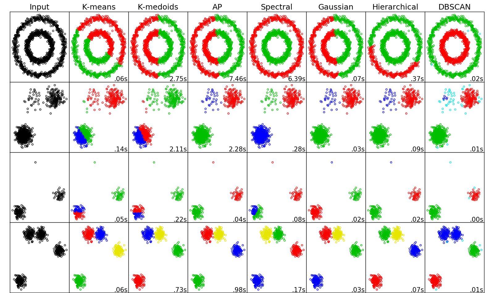
How to read the figure

The 4 rows represent 4 data sets with different structures: non-linear noisy circles, boxes with different densities, data with an outlier, and close boxes. The 6 columns represent input data plot, and results from k-means, k-medoids, Affinity Propagation, Spectral clustering, and Gaussian mixture clustering. Clustering results are shown with color labels: points drawn in same color are clustered in one group.

Spectral clustering beat other methods when the dataset has circular structure and boxes with different densities. For the second dataset, k-means and k-medoids often fails because random selection of center will prefer clusters with more points. For this dataset, Affinity Propagation sometimes works. The third dataset includes an outlier not far from the clusters, and Gaussian mixture model clustering does best at picking out the outlier. The last row is showing a dataset with four clusters, two of them are close to each other. All the algorithms do well, but the ways they partition the two close clusters are different.